LiCSAR File Structure and Products Details

Figure 1 shows the LiCSAR system file structure hierarchy. The blue parts represent the current state and the gray parts show the capabilities which will be available in the future. Starting from the top level, the LiCSAR products are categorized into 175 folders which corresponds to the Sentinel-1 175 orbits per cycle (for both Sentinel-1A and Sentinel-1B). In the next level, the frames are defined. The frames are slices that refer to the same point temporally and geographically. The name of each frame consists of 3 parts: in the first part, the three digits OOO denotes the orbit number while P shows whether it is descending (D) or ascending (A). The next part i.e. AAAAA shows the geographic location of the frame. Finally, the last part BBBBBB identifies the number of bursts where the the first, second and the third digit pairs identifies the number of bursts in the first, second and third sub-swath respectively.

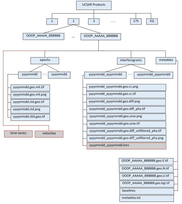
File structure of the LiCSAR system products

For each frame, the main LiCSAR outputs are stored in the ‘Products’ folder. As can be seen in Figure 1, all the generated interferometric pairs are located in the ‘Interferograms’ folder. The name of each interferometric pair shows the date of acquisitions in that pair. We are currently generating three interferograms per epoch. For the details of the LiCSAR methodology, the reader is referred to [1]. In summary, once a new acquisition arrives, it is being logically decomposed into pre-defined burst units and registered in the LiCSInfo database that handles burst and frame definitions. Images including bursts that form a given frame are extracted and merged into frame images. These are coregistered towards a primary frame image (a master image) that was set during the initialization of a frame, beforehand. The coregistration process includes the spectral diversity and other necessary corrections. Once coregistered, the interferograms are formed by combining the new image with three chronologically previous ones. This way is suitable for interpretation and for further use of the interferograms in multitemporal InSAR processing methods based on small baselines strategy (e.g. NSBAS approach currently implemented into custom LiCSBAS chain [2]). The interferogram unwrapping is performed using optimized SNAPHU approach. All the LiCSAR products are multilooked by factors of 5 in the range and 20 in the azimuth directions to achieve a resolution of around 100×100 m per pixel.

You can find the following datasets in each interferometric pair folder:

• geo.cc.tif: This is the coherence image of the interferometric pair. The values varies between 0-255 in which 0 refers to the lowest coherence values and 255 indicates the highest values of coherence.
• geo.diff_pha.tif: This is the wrapped phase image in radian. The values vary within the range of -3.14 to 3.14. These are differential phases as the topographic correction has already been applied using 1 arc-second SRTM DEM data.
• geo.unw.tif: This is the unwrapped phase image in radian. The unwrapping is performed using SNAPHU. The zero values in the unwrapped file refers to the pixels which are masked out due to the low coherence.

It should be noted that besides the original TIF files, the lower size PNG files were also generated in each folder. 

In addition to the interferograms, we have recently started archiving the multi-looked intensity images for each acquisition. These are located in the Epochs/yyyymmdd/Intensity. The intensity images are produced by space-domain averaging of the single look complex images.

We are also storing some other files in the Metadata folder. In this folder, the OOOP_AAAAA_BBBBBB.geo.E.tif, OOOP_AAAAA_BBBBBB.geo.N.tif and OOOP_AAAAA_BBBBBB.geo.U.tif files contain the east, north and upward components of the line-of-sight unit vector for each pixel. They are calculated from the SAR look-vector elevation and orientation angle of each pixel, based on the SAR imaging and DEM geometries with the local topography being taken into account. The unit vector information can be used, for example, to project E-N-U modelling results or 3-D geodetic observations like GNSS data onto the line-of-sight vector in order to be able to compare them to the LiCSAR results, or, to decompose line-of-sight displacement observations into east, north and upward components, if a scene is observed in more than one viewing geometry. The final two files in the Metadata folder namely OOOP_AAAAA_BBBBBB.geo.hgt.tif and OOOP_AAAAA_BBBBBB.geo.inc.tif refer to the extracted DEM and the incidence angle files for that frame respectively.

Atmospheric correction

We are currently developing an atmospheric correction module for the LiCSAR. The module is based on the Generic Atmospheric Correction Online Service (GACOS) model, developed at the University of Newcastle [3]. GACOS implements an iterative tropospheric decomposition interpolation model that decouples the elevation and turbulent tropospheric delay components.

As can be seen in Figure 1, the GACOS tropospheric delay maps will be provided in a grid binary format (yyyymmdd.ztd). Using the information provided in the yyyymmdd.hdr, the user will be able to read the binary file. The two key features of the GACOS products in the LiCSAR system are: (1) they are in the same resolution as of the other LiCSAR products (100×100 m), and (2) they are provided in the epoch Line Of Sight (LOS) direction. These features will allow the user to readily apply the correction to the LiCSAR phase products. This module will become available in June 2020.

Time-series

Finally, a time-series module is under development. This module is based on the LiCSBAS approach [2]. The main objective of this module is to generate the time-series results employing the LiCSAR products. The main outputs of the time-series module will be the velocity maps and the time-series displacements for all the frames. The products of the time-series module will be provided with 1 km resolution. This module will be available in September 2020.

References

1. Lazecky, M. et al. LiCSAR: An Automatic InSAR Tool for Monitoring Tectonic and Volcanic Activity, Remote Sens. 2020, https://doi.org/10.3390/rs12152430.
2. Morishita, Y.; Lazecky, M.; Wright, T.J.; Weiss, J.R.; Elliott, J.R.; Hooper, A. LiCSBAS: An Open-Source InSAR Time Series Analysis Package Integrated with the LiCSAR Automated Sentinel-1 InSAR Processor. Remote Sens. 2020, 12, 424.
3. Yu, C., Li, Z., Penna, N. T., & Crippa, P. (2018). Generic atmospheric correction model for Interferometric Synthetic
   Aperture Radar observations. Journal of Geophysical Research: Solid Earth, 123. https://doi.org/10.1029/2017JB015305